NYC Urban Ranger Animal Response

Let’s take a look at the data and see what types of animals have appeared in NYC!

data_raw <- read.csv("Urban_Park_Ranger_Animal_Condition_Response.csv")

#Animal by species
head(data_raw %>% count(Species.Description, sort =T))

##   Species.Description   n
## 1             Raccoon 497
## 2             raccoon  64
## 3        Canada Goose  37
## 4             Chicken  26
## 5     Red-tailed Hawk  25
## 6             Opossum  17

#Animal by classification
head(data_raw %>% count(Animal.Class, sort =T))

##                       Animal.Class   n
## 1                Small Mammals-RVS 582
## 2                            Birds 166
## 3                         Domestic  57
## 4                          Raptors  54
## 5            Small Mammals-non RVS  49
## 6 Terrestrial Reptile or Amphibian  21

Clearly, a lot of calls for raccoons! Unfortunately, this dataset does not include the reason for the call besides healthy, unhealthy, dead on arrival (DOA). There is some cleaning needed when looking at the classifications. Looking at $Marine Reptiles shows they’re actually $Terrestrial Reptiles. Let’s do some cleaning.

data_clean <- data_raw %>%
  mutate(
    Species.Description = str_to_lower(Species.Description), #removes capitializations
    Species.Description = str_replace_all(Species.Description, "-", " "), #removes dashes
    Animal.Class = str_to_lower(Animal.Class),
    Animal.Class = case_when(
      str_detect(Animal.Class, "marine reptiles") ~ "terrestrial reptile or amphibian", #moving turtles to correct category
      str_detect(Animal.Class, "marine mammals") ~ "marine mammals",
      str_detect(Animal.Class, "domestic") ~ "domestic",
      str_detect(Animal.Class, "raptors") ~ "raptors",
      str_detect(Animal.Class, "fish") ~ "fish",
      TRUE ~ Animal.Class),
    Species.Description = case_when(
      str_detect(Species.Description, "squirrel") ~ "squirrel", #more examples of this but this was most obvious
      TRUE ~ Species.Description
    )
  )

write.csv(data_clean, "UrbanRangerDataClean.csv")

Overall, this is much better now and solved some issues. I consolidated the Animal.Class category to make further analysis easier, but recognize this may have over simplified some details. There are some cases when some species are labelled different ways. We’ll leave this for now.

#Grouping by species for top 20 most abundant species
species <- data_clean %>%
  count(Species.Description, sort = TRUE) %>%
  top_n(20) 

## Selecting by n

#Species count
plot <- ggplot(data = species, aes(x= reorder(Species.Description, n), y = n)) + #reorder makes bars descending order
  geom_bar(stat = "identity") + #allows for the count to be plotted
  coord_flip() + #rotates graph
  labs(title= "Top 20 Species Count", y= "Count",x ="Species") + 
  theme_minimal() #introduces a theme to the figure instead of the standard output

plot

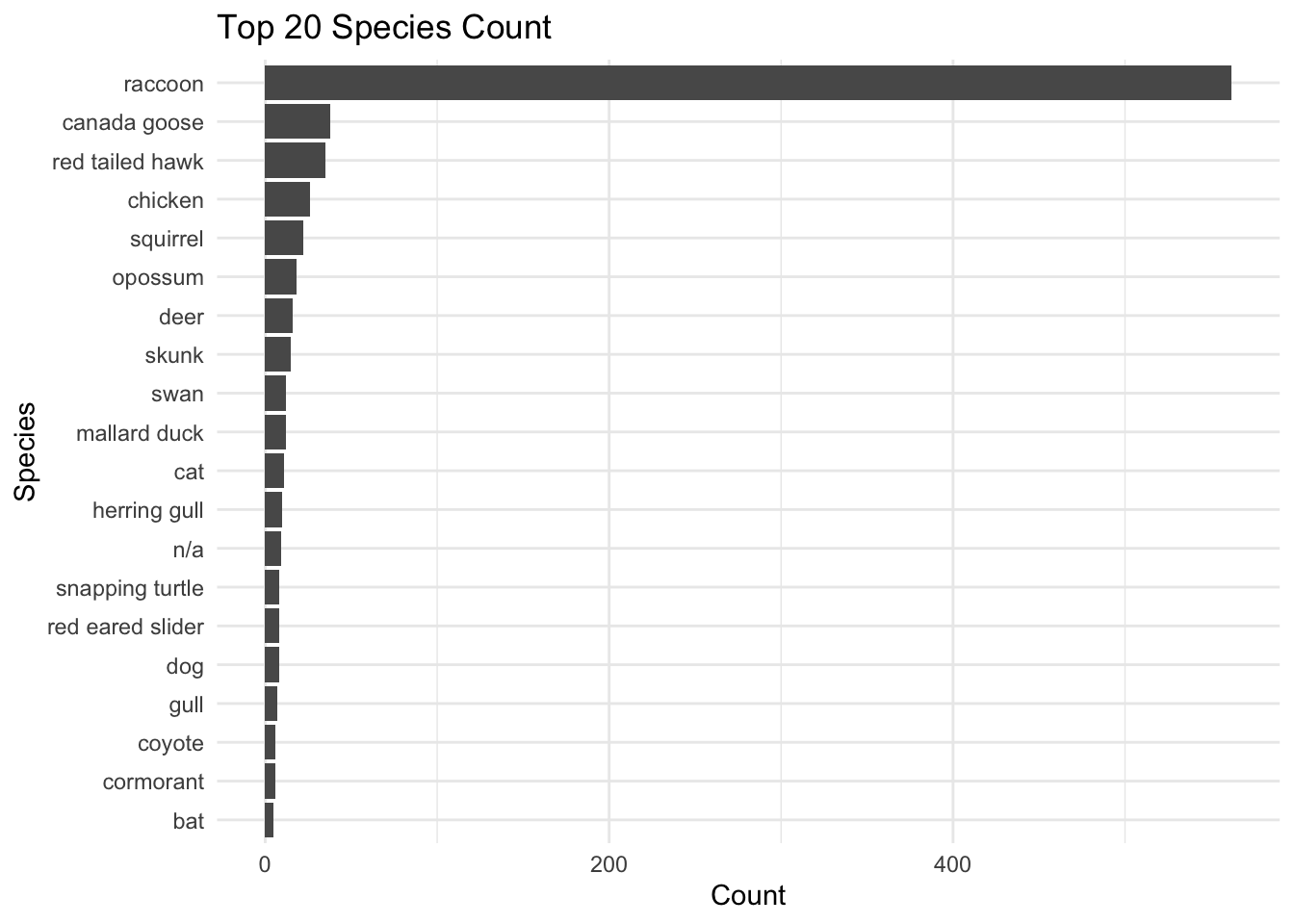
Funny to see that chickens are the fourth most reported animal in this dataset!

With such a high abundance of calls for raccoons, I’m going to remove them from the next graphic. This way we can understand how the rest of the species distributions look. Looking at how the Animal.Class reported across the boroughs.

plot2 <- data_clean %>%
  filter(Species.Description != "raccoon") %>%
  group_by(Borough) %>%
  count(Animal.Class, sort = TRUE)%>%
  ggplot(aes(x= reorder(Animal.Class, n), y = n)) + #reorder makes bars descending order, n represents count
  geom_bar(aes(fill=Borough), stat = "identity") + #allows for the count to be plotted
  scale_fill_brewer(palette = "Greens") +
  theme_classic()+ #introduces a theme to the figure instead of the standard output
  facet_wrap(~Borough, nrow=1)+
  labs(title = "Reports by Animal Classification, without raccoons", y= "Number of individuals reported", x=NULL)+
  coord_flip()

plot2

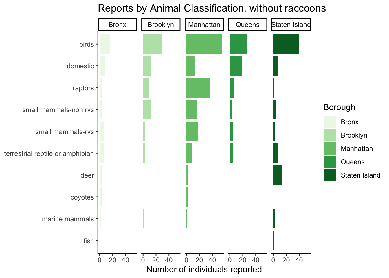
Now that we know that there are differences across the boroughs, let’s take a look at the most popular places animals are reported. Not surprising, this dataset falls within the NYC Parks most often.

plot3 <- data_clean %>% 
  count(Property, Borough, sort = TRUE) %>%
  top_n(10, n) %>%
  ggplot(aes(x=reorder(Property, -n), y=n)) +
  geom_bar(aes(fill = Borough), stat = "identity")+
  scale_fill_brewer(palette = "Greens")+
  xlab("")+
  ylab("Number of reported animals")+
  theme_minimal()+
  theme(axis.text.x = element_text(angle = 45, hjust = 1)) #rotates labels 45 degrees and adjust down to not overlap axis

plot3